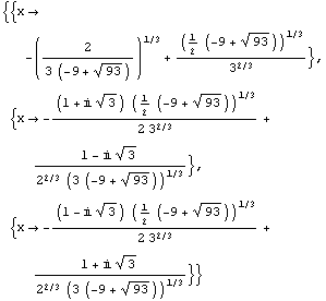
![(*1a*)Solve[x * x * x + x + 10, x] %//N](../HTMLFiles/ex02_solutions_127.gif)
Solution
In[44]:=
![(*1a*)Solve[x * x * x + x + 10, x] %//N](../HTMLFiles/ex02_solutions_127.gif)
Out[44]=

Out[45]=
![]()
In[46]:=
![(*1b*)Solve[{x * x + y * y1, y2x + 1}, {x, y}] %//N](../HTMLFiles/ex02_solutions_130.gif)
Out[46]=
![]()
Out[47]=
![]()
In[48]:=
![(*2*)Eliminate[{x + y + z0, x y z1, x/z2}, z]](../HTMLFiles/ex02_solutions_133.gif)
Out[48]=
![]()
See the help file for Eliminate for more info.
In[49]:=
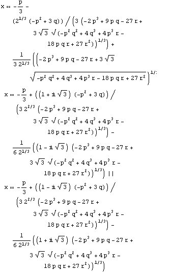
![(*3a*)Reduce[x^3 + p x^2 + q x + r0, x] ToRadicals[%]](../HTMLFiles/ex02_solutions_135.gif)
Out[49]=
![xRoot[r + q #1 + p #1^2 + #1^3&, 1] || xRoot[r + q #1 + p #1^2 + #1^3&, 2] || xRoot[r + q #1 + p #1^2 + #1^3&, 3]](../HTMLFiles/ex02_solutions_136.gif)
Out[50]=

Here Reduce produces Root-objects, which are roots of a pure function, with argument #1. The Root-objects can be converted into the usual form with the function ToRadicals. This works always for polynomials of order 4 or less.
In[51]:=
![]()
Out[51]=
![]()
In[52]:=
![]()
Out[52]=
![]()
The same as 3a with a further restriction on x.
In[58]:=
![(*3d*)Clear[a] Reduce[{x^3 - a x^2 + x - a0, x>0}, x] Reduce[{x^3 - a x^2 + x - a0, a>0}, x]](../HTMLFiles/ex02_solutions_142.gif)
Out[59]=
![]()
Out[60]=
![]()
Note that the symbols are treated as complex numbers unless they appear explicitly in an inequality, or the assumption Element[x,Reals] is made.
In[61]:=
![(*4*)Clear[a, b, c, d, e, x] Solve[a x * x * x * x + b x * x * x + c x * x + d x + e0, x]](../HTMLFiles/ex02_solutions_145.gif)
Out[62]=

In[63]:=
![(*5*)Solve[x * x + p x + 10, x] Plot[x/.%[[1]], {p, 2, 6}]](../HTMLFiles/ex02_solutions_147.gif)
Out[63]=

![[Graphics:../HTMLFiles/ex02_solutions_149.gif]](../HTMLFiles/ex02_solutions_149.gif)
Out[64]=
![]()
Remember how to apply rules, and extract an element from a list? The function Solve gives a list of rules for x. Then, when we apply the rule to x, we get an expression featuring p and q. Note that the discriminant of the equation is negative for p<2. Plot will complain if you try to plot it. There's a similar situation in the next excercise.
In[65]:=
![(*6*)Solve[x * x + p x + q0, x] f[p_, q_] = x/.%[[1]] Plot3D[f[p, q], {p, -15, 15}, {q, -15, 15}, AxesLabel {p, q, f}]](../HTMLFiles/ex02_solutions_151.gif)
Out[65]=

Out[66]=
![]()
![]()
![]()
![]()
![]()
![[Graphics:../HTMLFiles/ex02_solutions_158.gif]](../HTMLFiles/ex02_solutions_158.gif)
Out[67]=
![]()
In[68]:=
![]()
Out[68]=
![]()
SolveAlways tries to find the values of all free parameters appearing in an equation, here a, b and c, for which the equation holds for all values of the variable, here x.
| Created by Mathematica (April 10, 2007) |