Solution
The equation in question is y''(r)+V(r)y(r)=E y(r). The idea behind the matrix way of solving a differential equation is to consider the left hand side of this equation as an operator acting on the function y, i.e. L[y]=E y, and then transform the operator into matrix form with the method of finite differences. Then we have a matrix eigenvalue equation, denoted by M Y=E Y, which is easy to solve using a computer mathematics program. The eigenvectors of M, i.e. the vectors Y, are vectors with the values of the function y as their elements, i.e.  . The second derivative of y is transformed as
y''( )=
)= =
=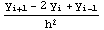 ,
,
so Schrödinger's equation in finite difference form looks like
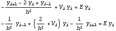
The idea is to form this equation at each of the points { }. Then we have a set of n linear equations for the variables
  , which can be written as M Y = E Y, and the elements of the matrix M are
  ="the coefficient of
  in the i:th equation". For example
  =-
=- ,
,  =
= +
+ . Most of the elements of M are zero. In fact, only the diagonal and the adjacent bands contain non-zero elements:
M=(
).
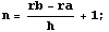
First, define the interval [ ,
, ] in which to search for the solution, and the spacing of the points {
 =
= ,
, =
= +h,
+h, =
= +2h,...,
 =
= } on this interval:
In[29]:=


The potential is of the form V(r)= +ε
+ε  , with ε=0.1. Calculate its values in points {
 }:
}:
In[33]:=

![V[r_] := r^2 + ϵ r^4 ;](../HTMLFiles/ex10_solutions_89.gif)
![vtab = Table[V[r], {r, ra, rb, h}] ;](../HTMLFiles/ex10_solutions_90.gif)
Then, construct the matrix M. The only non-zero elements for the ith row are  ,
,  and
and  .
.
In[36]:=
![M = Table[Switch[i - j, -1, -1/h^2, 1, -1/h^2, 0, 2/h^2 + vtab[[i]], _, 0], {i, n}, {j, n}] ;](../HTMLFiles/ex10_solutions_94.gif)
Now, the solutions of the equation M Y=E Y, the eigenvalues E and the corresponding eigenvectors Y can be calculated:
In[37]:=
![eigvec = Eigenvectors[M] ;](../HTMLFiles/ex10_solutions_95.gif)
![eigval = Eigenvalues[M] ;](../HTMLFiles/ex10_solutions_96.gif)
Then, we can plot the eigenfunctions, which can be obtained by means of interpolation.
In[39]:=

![Plot[Evaluate[Table[Interpolation[eigvec[[n - i]]][(x - ra)/h + 1], {i, 0, np}]], {x, ra, 5}, PlotRangeAll, PlotStyleTable[Hue[i/np], {i, 0, np}], ImageSize700] ;](../HTMLFiles/ex10_solutions_98.gif)
![[Graphics:../HTMLFiles/ex10_solutions_99.gif]](../HTMLFiles/ex10_solutions_99.gif)


