1. sin(x)
2. cos(x)
3.

4. Random[]
5. sin(cos(x)) and
 in the same figure.
6.
 (x),
(x),  (x),
(x),  (x), and
  (x) where
  (x)is the Bessel function of order n, given in Mathematica by the function BesselJ[n,x].
7. Try plotting the factorial function, n!.
Excercise 2
Plotting
Simple plots
Plot the following functions
1. sin(x)
2. cos(x)
3.
4. Random[]
5. sin(cos(x)) and in the same figure.
6. (x), (x), (x), and (x) where (x)is the Bessel function of order n, given in Mathematica by the function BesselJ[n,x].
7. Try plotting the factorial function, n!.
Parametric plots
1. Plot the curve x(t) =  +10t+1, y(t)=
 in x, y -coordinates.
2. Plot the curve (x(t), y(t)) = (cos(2 t),sin(π t))in x,y -coordinates.
3*. Plot the function z= , 0 < t < 2π on the complex z-plane, that is, in (Re z, Im z) coordinates. The functions Re[...] and Im[...] give the real and imaginary parts of a variable
3D and contour plots
1. Use Plot3D[...] and ContourPlot[...] to plot the following functions:
a.  , -5<x<5, -5<y<5
b. sin(x)cos(y)
Plot options
1. Using Mathematicas help system, find out how you can make coloured plots. Try it by plotting sin(x) and cos(x) to same figure with different colours. Can you also find a way to change the thickness of the lines?
2. Plot cos(2000 sin(x)), where 0<x<π. Find out how you can increase the number of points used in the plot to produce a better plot.
Additional excersises
1. Mathematica knows many special functions. Try plotting some of the following:
LegendreP[n,x], try with some integer values of n.
HermiteH[n,x]
LaguerreL[n,x]
MathieuC[a,q,x], try for example a=3, q=2
Zeta[s,a]
If you're interested, you can use the Mathematica help system to get more information about these functions.
2. Parametric 3D plot. Surfaces in three dimensions can be plotted by parametrizing the surface with two variables. As an example, try plotting the Möbius strip, given by the equations
![x(t, s) = [R + s cos(1/2t)] cos t y(t, s) = [R + s cos(1/2t)] sin t z(t, s) = s sin(1/2t)](HTMLFiles/ex02_solutions_66.gif) , 0≤t<2π, -w≤s<w,
, 0≤t<2π, -w≤s<w,
where R is the radius of the strip and w its width. Use Mathematicas built-in function ParametricPlot3D[{x, y, z}, {s, ,
,  }, {t,
  ,
, }], where x, y, and z are the coordinates and s and t are the parameters. Try different values of R and w.
Defining functions
1. Define the function f(x)=cos(10 sin(x))and plot it over x∈ [0,2π]
2. Define the function a(x,y) that calculates the average of two numbers x and y.
3. Define functions f(x)= , g(x)=exp(-x) and h(x) = g(f(x)). Plot the function over -5<x<5.
4. Define a function that computes  and plot it as a three dimensional plot.
5. Test the difference between delayed and direct assignment.
i. Set a=1
ii. Define the function f1(x)=exp(a x) using direct assignment ('=' operator)
iii. Define the function f2(x)=exp(a x) using delayed assignment (':=' operator)
iv. Plot f1(x) and f2(x) for 0<x<2.
v. Set a=1/2
vi. Plot f1(x) and f2(x) for 0<x<2.
Equations
Polynomial equations
1. Solve the following sets of equations symbolically, and find the numerical values of the solutions:
a.  +x+1=0
b.  +
+ =1,y=2x+1
2. Use Eliminate[...] to eliminate the variable z from the following set of equations

3. Use the function Reduce[...] to find the roots of the following equations:
a.  +p
+p  +q
+q  +r=0
+r=0
b. 
c. 
d. 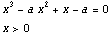
4. Find the general solution of a  + b
+ b  +c
+c  +d x+e=0. The result is really complicated!
5. Find the general solution of  +p x+1=0 and plot the first solution as a function of p.
6*. Find the general solution of  +p x+q=0, make a function f(p,q) that gives the first solution, and finally plot the function as a three dimensional plot, for -15<p<15, -15<q<15.
7*. Try what SolveAlways[...] does. Use it like Solve[...] on the second order polynomial equation a  +b x+c=0.
Algebraic equations
1. Use Solve[...] to find the solutions to the following equations
a.  =2
=2
b  =
=
c. 
d. x  =1
=1
e. x exp(exp(x)) = 1
2. Use Reduce[...] to find the solutions to the following equations
a.  +cos(x)=0
b.  +2
+2 -3=0
-3=0
3. Find the roots of the following equations. To get an initial guess for the solution, plot the right- and left-hand sides of the equations (or right-hand side minus the left-hand side alone) and make an estimate for the position of the root.
a. cos(x) = x
b. ln x=1/
c.  (x)=0, 5<x<6
 (x)is the Bessel J function, BesselJ[0,x] in Mathematica.
d. Define the function g(x)= exp(x sin(x))-x, plot it, and find its root.
Linear equations
Solve the following linear equations:
a. 
b.  +2
+2 +10
+10 =10,10
 +2
+2 +10
+10 =1,
=1, +2
+2 +3
+3 =0
=0
c. (
)(
1
2
3
0
1
2
0
0
1
)=(


)
1
1
1
d. (
)(
1
1
1
1
0
-1
2
1
0
)=(


)
0
1
2
Misc. equations
Solve the following equations. Choose an appropriate function (Solve, NSolve, FindRoot, LinearSolve)
a.  , a, b, c = ?
b.  , s, t, u = ?
c. x log(x)=10, x=?
d. sin(2x)+3 cos(x)+1=0, x=?
| Created by Mathematica (April 10, 2007) |  |